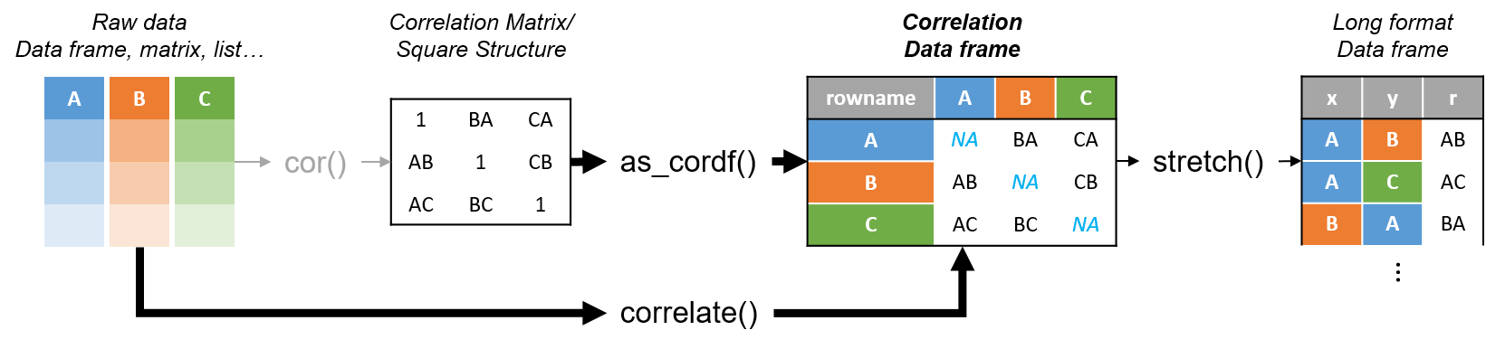
corrr is a package for exploring correlations in R. It focuses on creating and working with data frames of correlations (instead of matrices) that can be easily explored via corrr functions or by leveraging tools like those in the tidyverse. This, along with the primary corrr functions, is represented below:
You can install:
install.packages("corrr")# install.packages("remotes") remotes::install_github("tidymodels/corrr")Using corrr typically starts with correlate() , which acts like the base correlation function cor() . It differs by defaulting to pairwise deletion, and returning a correlation data frame ( cor_df ) of the following structure:
The corrr API is designed with data pipelines in mind (e.g., to use %>% from the magrittr package). After correlate() , the primary corrr functions take a cor_df as their first argument, and return a cor_df or tbl (or output like a plot). These functions serve one of three purposes:
Internal changes ( cor_df out):
Reshape structure ( tbl or cor_df out):
Output/visualizations (console/plot out):
The correlate() function also works with database tables. The function will automatically push the calculations of the correlations to the database, collect the results in R, and return the cor_df object. This allows for those results integrate with the rest of the corrr API.
library(MASS) library(corrr) set.seed(1) # Simulate three columns correlating about .7 with each other mu rep(0, 3) Sigma matrix(.7, nrow = 3, ncol = 3) + diag(3)*.3 seven mvrnorm(n = 1000, mu = mu, Sigma = Sigma) # Simulate three columns correlating about .4 with each other mu rep(0, 3) Sigma matrix(.4, nrow = 3, ncol = 3) + diag(3)*.6 four mvrnorm(n = 1000, mu = mu, Sigma = Sigma) # Bind together d cbind(seven, four) colnames(d) paste0("v", 1:ncol(d)) # Insert some missing values d[sample(1:nrow(d), 100, replace = TRUE), 1] NA d[sample(1:nrow(d), 200, replace = TRUE), 5] NA # Correlate x correlate(d) class(x) #> [1] "cor_df" "tbl_df" "tbl" "data.frame" x #> # A tibble: 6 × 7 #> term v1 v2 v3 v4 v5 v6 #> #> 1 v1 NA 0.684 0.716 0.00187 -0.00769 -0.0237 #> 2 v2 0.684 NA 0.702 -0.0248 0.00495 -0.0161 #> 3 v3 0.716 0.702 NA -0.00171 0.0205 -0.0566 #> 4 v4 0.00187 -0.0248 -0.00171 NA 0.452 0.442 #> 5 v5 -0.00769 0.00495 0.0205 0.452 NA 0.424 #> 6 v6 -0.0237 -0.0161 -0.0566 0.442 0.424 NANOTE: Previous to corrr 0.4.3, the first column of a cor_df dataframe was named “rowname”. As of corrr 0.4.3, the name of this first column changed to “term”.
As a tbl , we can use functions from data frame packages like dplyr , tidyr , ggplot2 :
library(dplyr) # Filter rows by correlation size x %>% filter(v1 > .6) #> # A tibble: 2 × 7 #> term v1 v2 v3 v4 v5 v6 #> #> 1 v2 0.684 NA 0.702 -0.0248 0.00495 -0.0161 #> 2 v3 0.716 0.702 NA -0.00171 0.0205 -0.0566corrr functions work in pipelines ( cor_df in; cor_df or tbl out):
x datasets::mtcars %>% correlate() %>% # Create correlation data frame (cor_df) focus(-cyl, -vs, mirror = TRUE) %>% # Focus on cor_df without 'cyl' and 'vs' rearrange() %>% # rearrange by correlations shave() # Shave off the upper triangle for a clean result #> Correlation computed with #> • Method: 'pearson' #> • Missing treated using: 'pairwise.complete.obs' fashion(x) #> term mpg drat am gear qsec carb hp wt disp #> 1 mpg #> 2 drat .68 #> 3 am .60 .71 #> 4 gear .48 .70 .79 #> 5 qsec .42 .09 -.23 -.21 #> 6 carb -.55 -.09 .06 .27 -.66 #> 7 hp -.78 -.45 -.24 -.13 -.71 .75 #> 8 wt -.87 -.71 -.69 -.58 -.17 .43 .66 #> 9 disp -.85 -.71 -.59 -.56 -.43 .39 .79 .89 rplot(x) 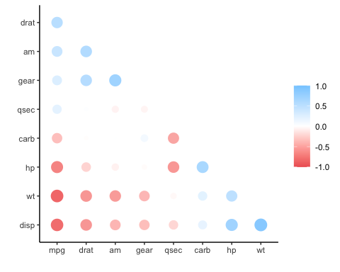
datasets::airquality %>% correlate() %>% network_plot(min_cor = .2) #> Correlation computed with #> • Method: 'pearson' #> • Missing treated using: 'pairwise.complete.obs' 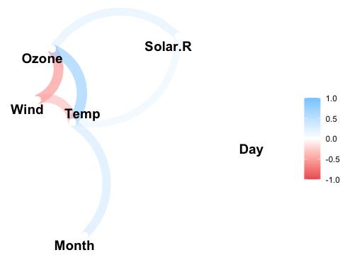
This project is released with a Contributor Code of Conduct. By contributing to this project, you agree to abide by its terms.